BioDynaMo User Guide

Written by Jean de Montigny

Introduction

BioDynaMo is platform for computer simulations of biological dynamics. You can learn more about BioDynaMo by accessing its official website.

This Tutorial in designed for user with limited knowledge of C++ language and will teach you the basics of BioDynaMo:

Create, build and run a new project
Create cells with a specific behaviour
Extend an existing structure
Visualize a simulation

Installation

You can access the installation page by clicking here.

Structure creation

As BioDynaMo is written is C++, it needs a particular structure. Fortunately, this procedure is really easy with BioDynaMo. To create a new project, you just need to run the command biodynamo new <project>. If you wish to have your Github account linked to your project you can append the --github option to the command. Try opening a terminal and running the command biodynamo new tutorial. This will create a folder named tutorial in your current directory, containing everything that BioDynaMo needs. Inside tutorial/src, two files with the basic structure already written have been created: tutorial.cc and tutorial.h. tutorial.cc will only contain the call to function Simulate which is defined in tutorial.h. This is were the core of our work will be added. You can easily compile your code using the command biodynamo build and run your simulation by typing the command biodynamo run. You can also directly use biodynamo demo tumor_concept to try this demo.

Cells and behaviors

The structure built in the previous chapter only creates a single cell. In this chapter we will create more cells in order to build a square of 2 400 randomly distributed cells. Afterwards, we will create a number of cancerous cells, that will grow and divide.

Creating cells

To do so, we will work only on the Simulate function of the tutorial.h file. First, we create a lambda function to set the simulation parameters programmatically. Second, we create a BioDynaMo simulation.

auto set_param = [](Param* param) {
  param->bound_space = Param::BoundSpaceMode::kClosed;
  param->min_bound = 0;
  param->max_bound = 100;  // cube of 100*100*100
};
Simulation simulation(argc, argv, set_param);

Afterwards, we obtain a reference to a few important objects.

ResourceManager will store our agents.
Random is a random number generator.
Param holds our simulation parameters.

auto* ctxt = simulation.GetExecutionContext();
auto* random = simulation.GetRandom();
auto* param = simulation.GetParam();

Let's define the number of cells we want to create and allocate three variables to hold the position (xcoord, ycoord and z_coord).

size_t nb_of_cells=2400; // number of cells in the simulation
real_t x_coord, y_coord, z_coord;

Then, with a simple loop from 0 to the number of cells, generate uniform distributed values for x, y and z and create a new cell object.

for (size_t i = 0; i < nb_of_cells; ++i) {
  // our modelling will be a cell cube of 100*100*100
  // random double between 0 and 100
  x_coord = random->Uniform(param->min_bound, param->max_bound);
  y_coord = random->Uniform(param->min_bound, param->max_bound);
  z_coord = random->Uniform(param->min_bound, param->max_bound);

  // creating the cell at position x, y, z
  Cell* cell = new Cell({x_coord, y_coord, z_coord});
  // set cell parameters
  cell->SetDiameter(7.5);

  ctxt->AddAgent(cell);  // put the created cell in our cells structure
}

We now have our structure containing all the 2400 cells! The code in charge of running our modelling is already written and will simulate it for only one step. Lets change this to simulate for 200 steps.

simulation.GetScheduler()->Simulate(200);

Behavior

In the previous chapter, we created a great number of cells. However, those cells don’t do anything! We will here create a cancerous cell that will grow and divide when it reaches a certain diameter. For this, we will define a new behavior structure Growth that will be applied to cell elements, and we will make this Growth copied into the cell daughter (so the daughter will also contain an instance of the behavior Growth)

struct Growth : public Behavior {
  BDM_BEHAVIOR_HEADER(Growth, Behavior, 1);

  Growth() { AlwaysCopyToNew(); }
  virtual ~Growth() {}

  void Run(Agent* so) override {
    // code to be executed at each simulation step
  }
};

We are now able to add any code in the Run() method, that will be executed at each simulation step for each cell containing this Growth. In our case, it will be a cellular growth, until a certain diameter is reached and then a cell division:

if (auto* cell = dynamic_cast<Cell*>(so)) {
  if (cell->GetDiameter() < 8) {
    cell->ChangeVolume(400);
  }
  else {
    cell->Divide();
  }
}

Of course, we need to create at least one new cell that contains our Growth behavior in our Simulate method

Cell* cell = new Cell({20, 50, 50});
cell->SetDiameter(6);
cell->AddBehavior(new Growth());
ctxt->AddAgent(cell);  // put the created cell in our cells structure

Run running it using biodynamo run. This code is now able to create and simulate 2 400 normal cells and 1 cancerous cell that will grow and divide! Complete code can be found in demo/tumor_concept.

Visualisation using Paraview

In the previous chapter we created a simulation of a great number of cell, also containing dividing cancerous cells, but we were not able to visualize anything, yet! In this chapter, we will set up visualization using Paraview (included in the BioDynaMo package). Dedicated page about visualization can be accessed here

Paraview

Paraview is an open source application for interactive and scientific visualisation. First of all, we need to tell BioDynaMo that we will use Paraview and so that we want the visualisation to be enable. To do that, we need to create a configuration file bdm.toml in the tutorial folder. Visualisation is of course not the only configuration we can do using this file. You can allow live visualisation (insitu=true) and/or export visualisation (here every 2 simulation step) by adding in bdm.toml

[visualization]
insitu = false
export = false
interval = 2

Afterwards, we have to define which agents will be considered for visualization:

[[visualize_agent]]
name = "Cell"

Because those visualization parameters are not in the source code, you don’t need to compile your code again. We can note that instead of creating a configuration file, you can do the same by creating this lambda function and passing it to the constructor of Simulation

auto set_param = [](auto* param) {
  param->insitu_visualization = true; // allows live visualisation
  param->export_visualization = true; // allows export of visualisation files
  param->visualization_interval = 2; // export visualisation files every 2 steps
  param->visualize_agents["Cell"] = std::set<std::string>{ "" };
}
Simulation simulation(argc, argv, set_param);

Once again, it is important to note that if you want to change any visualization parameter using this second method, you will have to compile your code again. That is not the case using a configuration file. Hence, using the toml file is highly recommended.

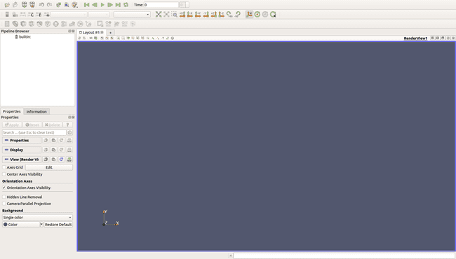
We will first have a look at export visualization then the live visualization. In both cases, simply run Paraview using the console line command paraview &. This window should appears

Export Visualisation (recommended)

In the configuration file (bdm.toml), turn the export parameter to true then run your modelling. You’ll notice the creation of several new files with the following file extensions *.pvsm, *.pvtu, *.vtu, *pvti, *.vti in the folder output/tutorial. Open ParaView and load the generated state file as described in Section Visualization (file -> load state)

A major advantage of export visualisation, in addition of not impacting the simulation time, is that you can visualise your modelling freely in time. using the arrows in the top menu, you can choose respectively to go back to the beginning of the simulation, go one step back, run normally, go one step further or go to the end of the simulation. You also can see witch step you are currently visualising (remember that this step number is the number of your modelling step divided by the export_interval you choose in your configuration file).

Live visualisation

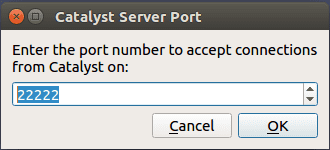
To use live visualisation, turn the insitu option of your configuration file to true, then click on the Catalyst top menu, and select Connect . This windows should appears

Click OK, then this windows should appears

Your Paraview is now accepting connections! Click OK, go back to the Catalyst menu, and select Pause Simulation. Using the same console, launch your tutorial simulation. You now notice that the programme stop right before running the simulation, because we used the Paraview Pause Simulation.

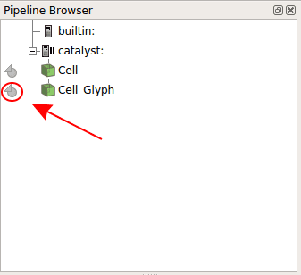
Go back to Paraview. You notice that new objects have appeared in the Pipeline Browser section. Click on the round shape in front of Cells Glyph.

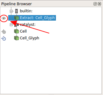
A new Builtin object have appeared: Extract: Cells Glyph. Click on the eye in front of it.

All cells appear on the screen! You can now go to the Catalyst menu, and select Continue. The simulation will run the number of steps you specified in your code.

Even if live visualization is particularly useful to set or tune a simulation, it is capital to note that it also drastically slows down the simulation! One way to avoid this major problem is to export visualization files and read then after the modeling is done.

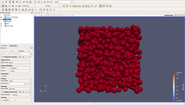
In both cases, even if we can now visualize our cell, they have all the same color, which can be a bit confusing and doesn't allow us to visualize properly what is going on.

Adding layers color

In this chapter, we will modify our code in order to create a better coloring for our simulation. A good idea would be to create a coloring depending on the layer of the cell. By this way, we could display several layers of cell, and have an other color for our cancerous cells. To do that, we can extend the existing Cell class in order to add a new data member cell_color. We will do that directly in our tutorial.h file by writing:

// 0. Define my custom cell MyCell, which extends Cell by adding extra data
// members: cell_color and can_divide
class MyCell : public Cell {  // our object extends the Cell object
                              // create the header with our new data member
  BDM_AGENT_HEADER(MyCell, Cell, 1);

 public:
  MyCell() {}
  explicit MyCell(const Real3& position) : Base(position) {}

  /// If MyCell divides, the daughter has to initialize its attributes
  void Initialize(const NewAgentEvent& event) override {
    Base::Initialize(event);

    if (auto* mother = dynamic_cast<MyCell*>(event.existing_agent)) {
      cell_color_ = mother->cell_color_;
      if (event.GetUid() == CellDivisionEvent::kUid) {
        // the daughter will be able to divide
        can_divide_ = true;
      } else {
        can_divide_ = mother->can_divide_;
      }
    }
  }

  void SetCellColor(int cell_color) { cell_color_ = cell_color; }
  int GetCellColor() const { return cell_color_; }

 private:
  // declare new data member and define their type
  // private data can only be accessed by public function and not directly
  int cell_color_;
};

Each cell (implementing our new object MyCell) of the modelling is now able to have a value cell_color_ that we will choose and use to display different colors! In order to create cells with this attribute, we need to replace all Cell object by MyCell during cells creation (inside the Simulate() method). For example

// Cell* cell = new Cell({x_coord, y_coord, z_coord});
MyCell* cell = new MyCell({x_coord, y_coord, z_coord});

Now that we are creating cells of type MyCell, we can set the cancerous cell cell_color_ value to 8 (so it will have a really distinct color from non cancerous cells). To do so, simply use the method SetCellColor() we created

cell->SetCellColour(8);

Do the same for the regular cells, setting the value depending on the y axis value. One possibility is to write

cell->SetCellColour((int)(y_coord / param->max_bound * 6)); // will vary from 0 to 5. so 6 different layers depending on y_coord

This new simulation is now functional, however before running it, we need to tell BioDynaMo to communicate all cell_color_ values. Do do that, we will modify the configuration file bdm.toml by modifying the visualize_agent

[[visualize_agent]]
name = "MyCell"
additional_data_members = [ "cell_color_" ]

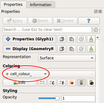
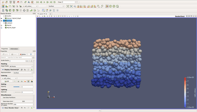
With those changes, we are now able to colorize our different layers. All you have to do, after displaying cells and creating the Glyph filter (chapter 3.1) is to select your Glyph filter and to select cell_color_ in the Coloring section.

Well done, we can now visualize the different layers and the cancerous cell in red!

However, there is still a little problem. The attribute cell_color_ is not transmitted to the daughter cell after a division. You can also notice that it is not really easy to see the cancerous cells. We will solve those issues in the next chapter.

Playing with filters

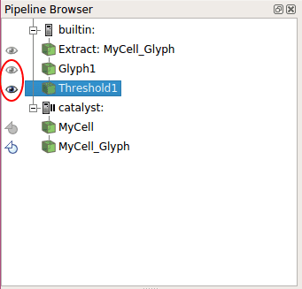
Even if our cancerous cells transmit their color to their daughter, it still is not really easy to spot them in the middle of thousands of other cells. This problem can be solve using the threshold filter function of ParaView. To do that, after displaying cells color as at the end of 3.2, click on the threshold filter button. This filter will be applied to the currently selected Pipeline Browser, so pay attention to select the correct one (Glyph1) before creating the threshold filter.

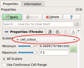
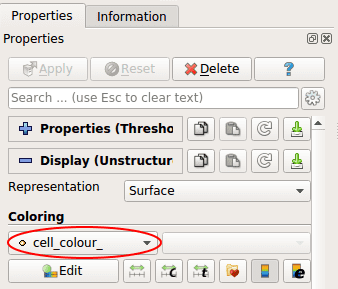
On the Properties menu, select the Scalar cell\colour_, put the minimum value at 7 and the maximum at 8 (so only the value of cancerous cell is selected) then click _Apply

Finally, choose the Coloring mode cell\colour__.

Great, we can now choose to display either all the cells, or just the cancerous cells by selecting either the Glyph1 or the Threshold1 in the Pipeline Browser!

This is of course just an example of what you can do with the threshold filters.

Adding some complexity

We now have all we want to visualize our modeling in the best conditions, but this modeling itself is a bit limited. We should add some movements to it as well as a new mechanism to complexity cell division. To add cell movement, we will modify the Run() method of our behavior Growth, and use the function UpdatePosition(). To generate the direction we will again use a random a random number generator. We choose here to give stochastic movement only to growing cells, so we will write the movement just after the volume change

auto* random = Simulation::GetActive()->GetRandom();
// create an array of 3 random numbers between -2 and 2
Real3 cell_movements =
    random->template UniformArray<3>(-2, 2);
// update the cell mass location, ie move the cell
cell->UpdatePosition(cell_movements);

Using the previous chapters, you should now be able to visualize cell movement during their growth. This is great, but every cancerous cell grows and divides indefinitely, and that is a bit too much. We will now add a mechanism to reduce the probability to divide, and assuring that a cancerous cell that didn't divide, will never divide any more. To add a 0.8 probability to divide, simply write

if (random->Uniform(0, 1) < 0.8) {
  cell->Divide();
}

Cells will now have only 80% chance to divide. However, it will have 80% chance to divide at every simulation step! We want that if a cell doesn't divide, it will not be able to divide any more. To do that, we will create a new MyCell boolean attribute called can_divide_, like we did for cell_colour_ attribute (see chapter 3.2).

BDM_AGENT_HEADER(MyCell, Cell, 1);

and create two methods, SetCanDivide() and GetCanDivide().

void SetCanDivide(bool d) { can_divide_ = d; }
bool GetCanDivide() { return can_divide_; }

Then, like we did for cell_colour_, declare this data member as private

bool can_divide_;

In the event constructor add the following lines to set can_divide_ to true in case of a CellDivisionEvent

if (event.GetUid() == CellDivisionEvent::kUid) {
  // the daughter will be able to divide
  can_divide_ = true;
} else {
  can_divide_ = mother->can_divide_;
}

Now that we got a new attribute can_divide_, we need to change the Run() method to prevent cells that failed the 80% test to divide again.

if (cell->GetCanDivide() && random->Uniform(0, 1) < 0.8) {
  cell->Divide();
} else {
  cell->SetCanDivide(false);  // this cell won't divide anymore
}

Codes corresponding to this chapter is accessible here.

You now have all the BioDynaMo cell basic knowledge to construct your own modeling!

Diffusion

Coming soon.

User Guide

Tumor Concept